This example shows how to use the bundled work block distribution together with the task context to handle situations where the work block can not hold the partitioned data because of a local memory size limit. The example calculates the dot product of two lists of large vectors as:
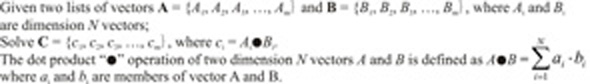
The dot product requires the element multiplication values of the vectors to be accumulated. In the case where a single work block can hold the all the data for vector Ai and Bi, the calculation is straight forward.
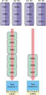
However, when the size of the vector is too big to fit into a single work block, the straight forward approach does not work. For example, with the Cell BE processor, there are only 256 KB of local memory on the SPE. It is impossible to store two double precision vectors when the dimension exceeds 16384. In addition, if you consider the extra memory needed by double buffering, code storage, and so on, you are only be able to handle two vectors of 7500 double precision float point elements each (7500*8[size of double]*2[two vectors] * 2[double buffer] ≈ 240 KB of local storage). In this case, large vectors must be partitioned to multiple work blocks and each work block can only return the partial result of a complete dot product.
You can choose to accumulate the partial results of these work blocks on the host to get the final result. But this is not an elegant solution and the performance is also affected. The better solution is to do these accumulations on the accelerators and do them in parallel.
- Implementation 1: Making use of task context and bundled work block distribution
- Implementation 2: Making use of multi-use work blocks together with task context or work block parameter/context buffers, with the limitation that accelerator side data partitioning is required
Source code
The source code for the two implementations is provided for you to compare with the shipped samples in the following directories:- task_context/dot_prod directory: Implementation 1. task context and bundled work block distribution
- task_context/dot_prod_multi directory: Implementation 2. multi-use work blocks together with task context or work block parameter/context buffers
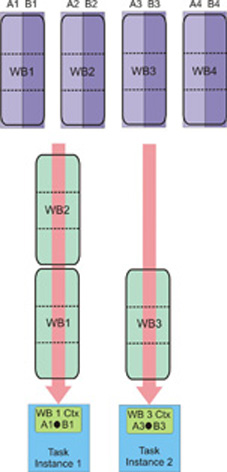
Implementation 1: Making use of task context and bundled work block distribution
For this implementation, all the work blocks of a single vector are put into a bundle. All the work blocks in a single bundle are assigned to one task instance in the order of enqueuing. This means it is possible to use the task context to accumulate the intermediate results and write out the final result when the last work block is processed.
The accumulator in task context is initialized to zero each time a new work block bundle starts.
When the last work block in the bundle is processed, the accumulated value in the task context is copied to the output buffer and then written back to the result area.
Implementation 2: Making use of multi-use work blocks together with task context or work block parameter/context buffers
The second implementation is based on multi-use work blocks and work block parameter and context buffers. A multi-use work block is similar to an iteration operation. The accelerator side runtime repeatedly processes the work block until it reaches the provided number of iteration. By using accelerator side data partitioning, it is possible to access different input data during each iteration of the work block. This means the application can be used to handle larger data which a single work block cannot cover due to local storage limitations. Also, the parameter and context buffer of the multi-use work block is kept through the iterations, so you can also choose to keep the accumulator in this buffer, instead of using the task context buffer.