Final Results

Here are the final results from the study. Click here for the final report.

Description Precision # Cells Walltime (s) Speed-up Comm/Comp Efficiency
CPU double 160×80 200
1 GPU double 640×320 737 17.2
1 GPU single 640×320 642 19.8
2 GPU double 2560×1280 29,750 27.5 0.098 0.80
2 GPU single 2560×1280 19,180 42.6 0.066 1.08
4 GPU double 2560×1280 19,005 42.9 0.38 0.62
4 GPU single 2560×1280 11,750 69.4 0.27 0.88
8 GPU double 2560×1280 12,659 64.1 0.81 0.47
8 GPU single 2560×1280 7,341 110.7 0.52 0.70

Below are some links to animations of the simulations performed for the above table.
160×80 Single Precision
160×80 Double Precision
640×320 Single Precision
640×320 Double Precision
2560×1280 Single Precision
2560×1280 Double Precision

Future work includes improving the efficiency of the MPI by performing domain decomposition in 2 dimensions and not just one. Also, there will be some working with memory efficiency to boost the speed-up of single precision. Finally, parallel I/O will be necessary at some point because output is really becoming a bottleneck.

Overall, I was happy to see the 64x speed-up in double precision, even if it took 8 GPUs to obtain it at below half efficiency per GPU. The main reason for poor MPI efficiency is network bandwidth which is evidenced by the fact that single precision (which has less computation per time step) had a lower communication to computation ratio. This is evidence that bandwidth is the main limiter of communication time. A higher bandwidth interconnect would help the situation.

Given these results (with some “back of the envelope” calculations) and the vast room for improvement that still remains, I am genuinely optimistic about the potential use of GPUs for real atmospheric simulation in 3-D. Probably the biggest motivator is getting at least 10-20x more computational power for the money compared to CPUs.

There main question I have at this point is: how well would physics packages transition to GPU kernels given a reasonably large amount of “if/then” logic in some of the modules? I doubt the memory will be a restriction because 1Gb is a very large amount of memory. With a required memory for 150 variable and 150 fluxes on a grid of N^2 cells, 1800×1800 cells can be simulated, which is more than would ever be places on a single GPU in MPI domain decomposition. If divergent control flow can be altered or handled efficiently, then GPUs deserve a good hard look by the atmospheric community.

Serial Optimizations and Asymmetry Fixed

I have several updates regarding the project.

Optimizations
First, it occurred to me that I had not really optimized the serial code for the CPU it was running on. The CPU has 2 cores, and I had not inserted OpenMP pragmas into the code to take advantage of that. So I put in OMP parallel for pragmas before the outer loop of every subroutine that is looped in the main time step while loop: flux_x, update_x, flux_z, update_z, source, and boundaries. I tried with OMP_NUM_THREADS set to 1, 2, and 4. The optimal value on this processor was 2, and it came very close to a speed-up of 2.

I also made an optimization to both the serial and CUDA codes where I took out a pow(…,2) and performed the squaring with multiplication instead. Evidently pow() takes a lot of cycles to complete because the runtimes were substantially lower. Because of this observation, I took pains to remove as much duplication of pow() statements (in both serial and CUDA codes) as possible, and this further reduced the runtime quite a bit. The serial code which previously ran at 460 seconds now runs at 198 seconds.

Code Corrections
I finally found the reason for the asymmetry in my results. It was a surprisingly bad error that gave surprisingly realistic results. In the flux computation, I perform Gaussian quadrature to integrate over an interval. I made the mistake of integrating out over the wrong interval, so when I fixed this, the solution was finally symmetric (at least in double precision). I realized that single precision does lead to some pretty pronounced asymmetries, so I changed my mind again and decided the solution must be in double precision for accuracy purposes. The flow I am using for the project is turbulent, and in turbulent (and therefore chaotic) flows, any (even machine precision) difference will amplify into visible differences later in the solution. The classic example of this is the Lorenz attractor.

CUDA-Specific Optimizations
I’ve had some fairly surprising results as far as CUDA optimizations in general. First, running with a maximum of 128 registers allocated per thread (via a compiler flag) and using 128 threads per block (16×8) was actually slower than running with 64 registers per thread and 256 threads per block (16×16). The reason this is surprising is that running with 64 registers actually uses significantly more local memory (which is very slow and uncached) in a given thread than running with 128. Evidently, 256 threads better hides the memory latency and better fills the device.

I also discovered the joys of loop unrolling with the #pragma unroll directive. I found that the compiler will not unroll a loop if the pow() function is called. It complains that unexpected control flow occurred and refuses to unroll. The faster yet less accurate __powf() function will work with unrolling, but not the pow() function. After some testing, I concluded that the inaccuracy due to the CUDA __powf() function was not worth the performance gain. Even though the loop unrolling increased the amount of local memory used, it gave an 8% gain in efficiency.

New Speed-Up Values
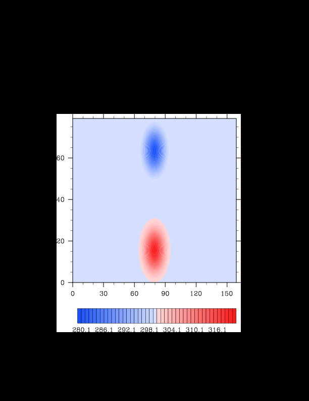
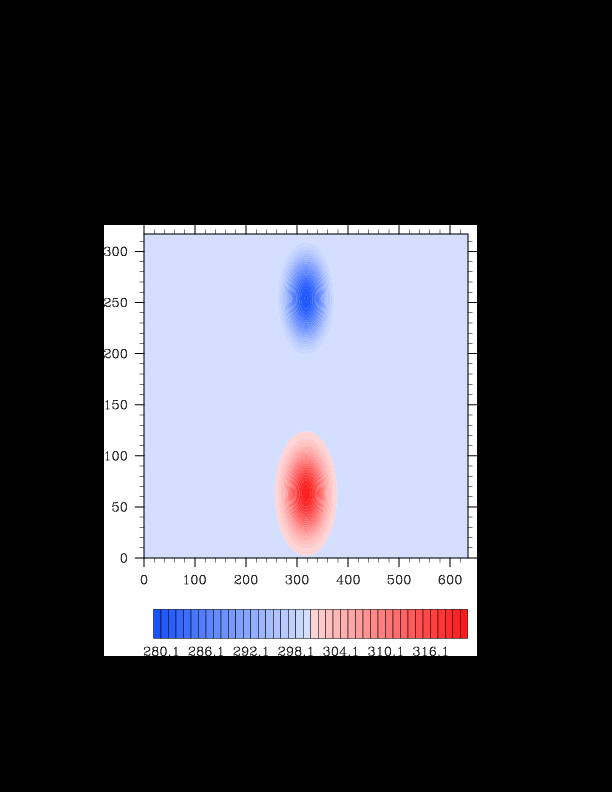
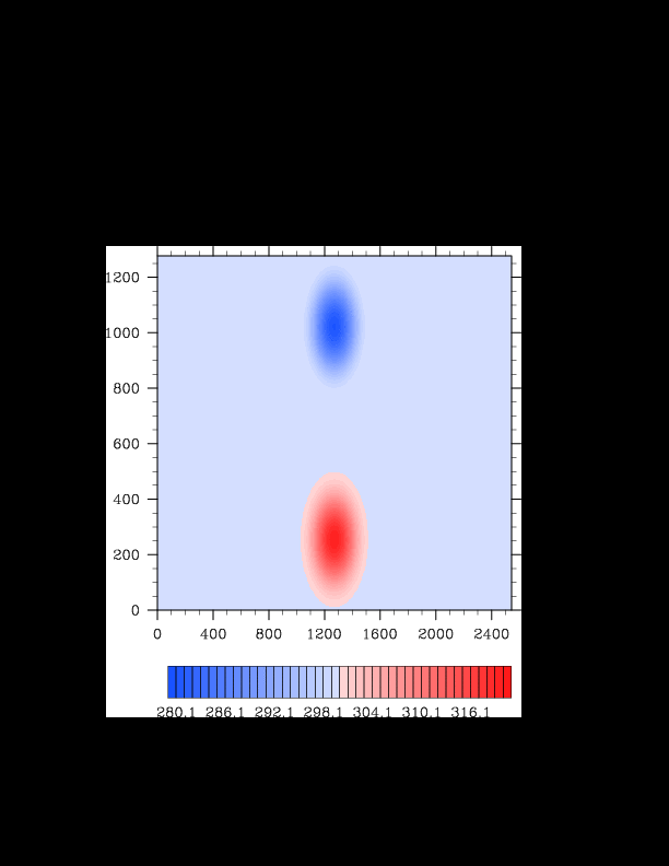
With the new optimizations, the serial code on a 160 x 80 grid runs in 198 seconds. The double precision CUDA code on a 680 x 320 grid runs in 736 seconds. This gives a speed-up of just over 17x on a single GPU. It is apparent that 4 GPUs will not give the 64x speed-up I wanted from the beginning because from prior experience, the speed-up is highly sub-linear for small problems. I may need to go to 1360 x 640 to get that speed-up on 4 GPUs. Because there is less computation in the kernel available to hide memory latency, the single-precision CUDA version only gave a 24x speed-up. Relative to the double precision speed-up, this is less than before. So the speed advantages of going with single precision are less pronounced.

Overall Thoughts for Single-GPU Optimizations
For a scientist who is interested in a good speed-up without the hassle of overly tedious optimizations, I would say to pay attention to the following:

  • Make sure you have enough threads per block to hide memory latencies (at least 128, but 256 may be better)
  • Make sure you have enough blocks to fill the device. On the GTX 280, there are 3 clusters of 10 SMPs which means you need at least 30 blocks, but preferably many, many more.
  • If you have read-only constants, declare them as __shared__, making sure you don’t overflow the available 16Kb per block. Use the -Xptxas compile flag to output to console how much shared memory a kernel will use per thread (multiply this by the number of threads per block in the kernel launch for total shared memory use).
  • Unroll loops whenever possible. I doubt you’ll overflow local memory.
  • For me, it was worth it to run 256 threads per block rather than 128 if possible. Use the compile flag –maxrregcount to limit the number of registers per thread. You have 16K registers per block and 16Kb of shared memory per block on the GTX280, so ensure on your specific GPU to obey its constraints. I tried –maxrregcount 32 with 512 threads per block, but this was slower than 256 threads per block.
  • If you can use single precision, do so. It will likely be a factor of 2x faster than the speed-up with doubles. But make sure it doesn’t unacceptably degrade accuracy.

Obviously if you have a linear algebra issue, don’t reinvent the wheel. Use cuBLAS or something similar. But if you have a kernel with fairly simple (and repeated) access to global memory, go ahead and coalesce the reads into shared memory and work within shared memory. In my case, it simply wasn’t worth the effort because the code would have become very difficult to understand and maintain. If it’s not simple, I say just let the compiler coalesce your reads for you and work in global memory. If your global memory ends up in local variables, and most of your kernel works on those local variables (as was the case with my main kernels), I have to believe the compiler is smart enough to know to allocate those variables as registers, so it may not be beneficial to explicitly declare them as shared. In fact, when I tried to do this, it degraded performance.

As for porting code to the GPU. If you have a loop structure like

for (i = 0; i < NX; i++) {
    for (j = 0; j < NY; j++) {

It is easiest to convert it for use in a kernel as

ii = blockIdx.x*blockDim.x + threadIdx.x;
jj = blockIDx.y*blockDim.y + threadIdx.y;
for (i = ii; i < NX; i+=gridDim.x*blockDim.x) {
    for (j = jj; j < NY; j+=gridDim.y*blockDim.y) {

This way, you know all of the work is getting done, and it places the burden of optimization on ensuring that NX and NY are multiples of 32 or have a division remainder as close to 32 as possible to make sure all warps are optimally productive.

GPU + MPI Successfully Implemented!

I have finally implemented a CUDA + MPI model and have run it on 4 GPUs successfully. I also decided to switch to single precision against my previous conclusions because I realized the asymmetry is because of my code. I have yet to track that one down, but it doesn’t affect the compute time aspects relevant to this class project. Running in single precision, the speed-up jumped from 18 to 37.5 which shows that these GPUs really were meant for single precision.

Running on 4 GPUs at quadruple the standard test case resolution, the total speed-up was 65.5 which is an effective speed-up of only 16 per GPU. This is attributed to several aspects including replicated work at domain decomposition boundaries, DMA+network transfers of boundaries between GPUs, and not filling the devices fully because of too little data to work on per GPU. So I halved the grid spacing (which should take 512 times longer than the standard test case in serial) to increase the workload per GPU, hide the relative memory latency between devices, and reduce the relative amount of replicated work. This simulation gave a speed-up of 98 which was a speed-up of about 25 per GPU (a big improvement). This goes to show that you really need to do more work per GPU (solve bigger problems) to get the desired speed-up, and this is no problem for me :) .

At this point, I will likely call the project finished unless prompted otherwise by the instructor. I got my desired speed-up of 64 and then some. My impressions of GPUs for scientific computing are very positive at this point. Unfortunately, many geophysical codes (especially physics modules in atmospheric codes) have diverging control flow and very high memory requirements. If the memory can be effectively mapped to GPUs and if the diverging control flow either avoided or intelligently handled, I think they may actually find a place in climate codes eventually. This is no easy task though.

Effects of Doubling Resolution

Just to give a visual notion of the effects of doubling resolution on a particularly active flow (buoyancy-driven density current in a neutral atmosphere), consider the following two plots of potential temperature 900 seconds after a cold bubble was released toward the ground (somewhat similar to a small-scale front). I’m not sure if the solution to this particular flow is going to converge on large scales as the mesh and time step are refined. My hunch is that it will but that much finer resolution is necessary to do so. Note that this is not the typical Straka test case because no physical dissipation (e.g. eddy viscosity) is included in the model as of yet. The resolution of secondary Kelvin-Helmholtz type waves is impressive in just a doubling of resolution. This is likely manifesting the 3rd- to 5th-order convergence of the WENO spatial interpolant.

The normal resolution is 50m in both the x and z directions on a domain of 53km x 6.4km. This gives about 135,000 cells to simulate. The doubled resolution simulates 4 times as many cells at half the time step, simulating over 500,000 cells. The standard resolution which typically took several hours on my CPU took only 10 minutes on the GPU, and the doubled resolution took just over an hour. As with the bubble test case from the previous post, theoretically, the doubled resolution should take 8 times longer to run, but it only took 7 times longer on the GPU. I would attribute this to hiding the overhead of kernel invocation and memory latency by doubling the per-thread work. At the current speed-up, it would take in the ballpark of 9-10 hours to simulate a quadrupled resolution on a GPU. I hope to cut that down to roughly 2.5 hours in the MPI+GPU version of the code with 4 GPUs.

straka_normalres

straka_doubleres

I realized that I didn’t post any pictures of the bubble experiment. The following two pictures are standard and quadrupled resolution versions of the rising thermal test case with a linear perturbation in the domain center near the ground. The bubble rises for 1,000 seconds. The resolution requirements for the standard test case were small enough that it was more than feasible to get a quadrupled resolution out of the GPU. The standard grid spacing is uniformly 125 meters, giving a quadrupled grid spacing of about 30 meters.

bubble_normalres

bubble_quadres

Success! A Working CUDA Implementation

After reworking the code again, I have successfully completed a CUDA implementation for GPGPUs with surprising results. On a single CPU, I was able to perform reconstruction, flux computation, and updating all in one step. However, because blocks cannot communicate, I had to split this operation into two kernels. The first kernel handles reconstruction and flux computations, and the second performs the updating. There are 5 kernels in all:

1. Perform reconstruction and flux computations in the x-direction

2. Perform reconstruction and flux computations in the z-direction

3. Update state variables in the x-direction

4. Update state variables in the z-direction

5. Update the domain boundaries to satisfy boundary conditions

Each kernel is left with almost identical code as the serial version except that the loop is broken up by threads. This ensures that all of the work gets done, and it is up to proper specifications of gridDim and blockDim to optimize GPU occupancy.

The domain for the convective bubble experiment is typically 160 x 80 cells which can be very naturally divided into a 10 x 10 grid of blocks with 16 x 8 threads a piece. From my “back of the envelope” calculations, 128 threads per block shouldn’t produce pressure on the per-block register space, and it hides memory latency efficiently according to nvidia’s documentation. To double the resolution, I simply invoked a 20 x 20 grid of the same sized blocks to accomplish the work and get more occupancy out of the GPU. Theoretically, doubling the resolution should result in 8x more wall time, but on the GPU, it only took 7x longer which I attribute to hiding more of the memory latency.

Overall, the speed-up (compared to my mediocre workstation CPU) is 18x. To put numbers to this, a simulation which took around 10 minutes on my CPU takes around 30 seconds on a GPU. I found this extremely surprising because I’m using double precision and haven’t performed any memory optimizations at all. Every access is to global memory or register memory (no shared accesses), and I haven’t paid attention to any bank conflict issues yet. The nvcc compiler automatically attempts to coalesce global memory accesses, but I do not believe it pulls anything into shared memory for repeated accesses. This indicates that some extra speed-up is available through memory optimizations.

I will not be optimizing memory any further for the present class project, however, because it is more fruitful in the immediate to go ahead and pursue a GPU+MPI implementation. My original goal was to achieve a combined 64x speed-up over my workstation CPU running in serial which would allow a quadrupling of model resolution. I thought this was overly ambitious in the beginning, but I now think it is more than feasible.

Successfully Ported to C

True to scientist’s time, I have finally finished a successful port to C from Fortran 90 a day later than I planned to have the port and a basic CUDA kernel ready. However, the delays were for a good reason.

I found a way to reduce all of the work for a time step into two function calls (instead of six) which reduces the number of kernel launches by 1/3 and significantly reduces the required memory. The original algorithm first performed reconstruction and stored it into memory (nx * nz * 20 doubles required). Then, these reconstructions are integrated over to compute the fluxes which are stored into memory (nx * nz * 4 double required). Finally, the fluxes are used to update the cells. In the new algorithm, the reconstructions, fluxes, and updates are all performed in one step to increase the amount of computation in a single kernel call. Also, the memory requirements are reduced by a factor of 7 which should be more suitable for the GPU.

These changes were made, most importantly, without any branching logic. The next step is to convert the 2 functions calls (one for the x-direction, one for the z-direction) into CUDA kernels.

I ran some tests to experiment with single precision. Using a typedef, I implemented a compile time directed switch between single and double precision. Single precision causes significant artifacts in terms of violating spatial symmetry, particularly near the boundaries. Therefore, for correctness purposes, the luxury of single precision will not be possible for this particular algorithm without identifying where cancellation is occurring.

Welcome

Welcome to my course project webpage where you can keep up with my progress on parallelizing a 2-D Dry Inviscid Compressible Non-Hydrostatic Atmospheric Model for GPGPUs (General Purpose Graphical Processing Units) using Nvidia’s CUDA language.

website_graphic

My name is Matthew Norman. I’m a Ph.D. student in the Marine, Earth, & Atmospheric Sciences department at North Carolina State University under the Department of Energy Computational Science Graduate Fellowship.

The project proposal is also available for viewing.